How to Build a Shipping Analytics Dashboard in Power BI
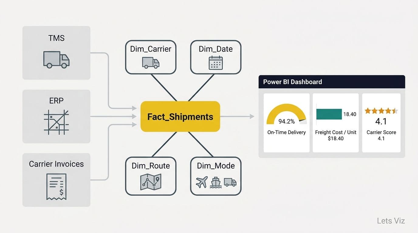
Building a shipping analytics dashboard in Power BI means connecting your TMS, ERP, and carrier invoice data into a star schema, defining three core KPIs - on-time delivery rate, freight cost per unit, and carrier performance score - and writing DAX measures and drill-through pages on top. Most mid-market teams reach a working version one in four to six weeks. The same architecture also powers patient flow analytics dashboards in Power BI for health systems tracking bed occupancy and discharge bottlenecks - covered in a dedicated section below, along with a step-by-step guide to building an emergency department analytics dashboard in Power BI with HIPAA, GDPR, and PIPEDA-compliant data handling. Teams already in the Zoho ecosystem can follow the same KPI framework inside Zoho Analytics; a dedicated section below covers how to build a dashboard in Zoho Analytics step by step.
Key Takeaways
Three KPIs anchor every logistics dashboard: on-time delivery rate, freight cost per unit, and carrier performance score.
Your choice between Import Mode and DirectQuery determines refresh latency and DAX compatibility.
SUMX and CROSSFILTER are the two DAX functions used most in freight cost models.
Carrier-level drill-through pages turn an executive summary into an operational tool.
Row-level security must be configured before publishing to operations and finance teams.
Lets Viz specialises in Power BI for SaaS finance teams - from MRR waterfall and cohort retention to board-ready financial dashboards.
What KPIs Should a Shipping Analytics Dashboard Track?
On-time delivery rate, freight cost per unit, and carrier performance score form the essential baseline. Before writing a single DAX measure, align with your CFO or VP of Operations on which three metrics will appear in the weekly ops review. Everything else belongs on a drill-through detail page.
On-time delivery rate = shipments delivered on or before the promised date divided by total shipments. The 95-99% range is a standard B2B benchmark; CPG retail replenishment typically demands 98% or higher. Track this as both a percentage and an absolute count of late shipments so operations managers see business impact alongside the rate.
Freight cost per unit = total freight spend divided by total units shipped. Breaking this KPI by carrier, lane, and mode (full truckload, LTL, parcel) reveals where negotiation leverage exists and where mode shifts can deliver savings.
Carrier performance score is a composite of OTD rate, damage rate, and invoice accuracy, optionally weighted by shipment volume. A single number per carrier makes the executive summary scannable in under 30 seconds.
The table below maps each KPI to its formula, target range, and best drill dimension.
| KPI | Formula | Target Range | Primary Drill Dimension |
|---|---|---|---|
| On-Time Delivery Rate | On-time shipments / Total shipments | 95-99% | Carrier, Lane, Month |
| Freight Cost per Unit | Total freight spend / Units shipped | Varies by mode | Carrier, SKU, Region |
| Carrier Performance Score | Weighted composite (OTD, damage, invoice) | 85-100 | Carrier, Quarter |
| Average Transit Time | Sum(transit days) / Total shipments | Lane benchmark | Origin-Dest pair |
| Damage / Exception Rate | Damaged shipments / Total shipments | Below 0.5% | Carrier, Product |
For a broader framework on structuring KPI hierarchies across finance and operations dashboards, what metrics should a financial reporting dashboard include covers the selection methodology in detail.
How Do You Connect and Model Shipping Data in Power BI?
Most logistics teams pull from three source systems: a TMS (Transportation Management System), an ERP or order management system, and carrier invoicing portals. The connection method depends on what each source exposes - SQL database, REST API, or CSV/Excel export. Use Power Query to build one clean query per source table and land everything in a star schema inside Power BI Desktop.
FactShipments is your central fact table - one row per shipment:
ShipmentID, OrderID, ShipDate, DeliveredDate, PromisedDate
FreightCost, UnitsShipped, WeightLbs
CarrierID, LaneID, ProductID (foreign keys to dimensions)
Dimension tables to build:
DimCarrier - CarrierName, Mode (FTL/LTL/Parcel), Region
DimDate - built with `CALENDARAUTO()` or a pre-built static table; mark it as a date table in the model
DimLane - OriginCity, DestCity, DistanceMiles, DistanceBand
DimProduct - SKU, Category, WeightClass
Keeping foreign keys clean - no mixed CarrierID formats, no nulls in ShipDate, no mismatched lane codes between your TMS and ERP - removes the majority of DAX debugging time later. Run a data quality check in Power Query before building any measures: count distinct values in each key field and flag anomalies before they produce incorrect KPIs on a live dashboard.
According to the World Economic Forum (2026), over 100 experts representing more than 50 financial services and operations organizations identified operational data integration as the top barrier to analytics adoption. Logistics teams face the same friction - mismatched carrier codes and inconsistent date fields between TMS and ERP systems are the most common cause of dashboard rework.
The patterns used for financial fact table modeling transfer directly here. Automating monthly financial reporting in Power BI covers star schema design and date table conventions that apply equally to logistics datasets.
How to Build a Shipping Analytics Dashboard in Power BI: Import Mode vs. DirectQuery
Your data architecture choice is the most consequential technical decision you will make before writing a single measure. Import Mode loads a compressed snapshot into Power BI's in-memory engine (VertiPaq), delivering sub-second query performance and supporting the full DAX library. DirectQuery queries your source database live on every user interaction, keeping data real-time but adding latency and restricting certain DAX patterns.
For most shipping dashboards, the decision follows a clear rule:
Choose Import Mode when:
Your shipment fact table has fewer than 50 million rows
A daily or hourly scheduled refresh fits operational needs
You need the full DAX library (SUMX, CROSSFILTER, time intelligence functions are all supported)
Choose DirectQuery when:
You need real-time same-day shipment status with sub-hour latency
Your source database has indexed CarrierID, ShipDate, and LaneID
You can accept that complex calculated columns and some DAX iterator patterns are unavailable
A hybrid approach - Import Mode for 13 months of historical data, DirectQuery for a live "today's shipments" table - is supported via Power BI composite models. This is the architecture most mid-market logistics teams settle on when they need both a trend view and a real-time operational screen.
The Power BI financial reporting dashboards guide covers Import Mode vs. DirectQuery trade-offs in the context of finance fact tables, which share the same volume and refresh constraints as logistics data and offer useful analogies for the architecture decision.
How Do You Write DAX Measures for Freight Cost and On-Time Delivery?
Two DAX functions carry most of the weight in a freight cost model: SUMX (an iterator function) and CROSSFILTER.
SUMX calculates a value at the row level before aggregating - essential when shipment sizes vary widely:
```dax
Freight Cost per Unit =
SUMX(
FactShipments,
DIVIDE( FactShipments[FreightCost], FactShipments[UnitsShipped], 0 )
)
```
A simple `SUM(FreightCost) / SUM(UnitsShipped)` produces an average of averages, which overstates cost for small, expensive parcel shipments relative to high-volume FTL lanes. SUMX respects the row-level division before rolling up, making it the correct pattern for any per-unit cost measure.
For on-time delivery rate, the COUNTROWS/FILTER pattern is standard:
```dax
On-Time Delivery Rate =
DIVIDE(
COUNTROWS( FILTER( FactShipments, FactShipments[DeliveredDate] <= FactShipments[PromisedDate] ) ),
COUNTROWS( FactShipments ),
0
)
```
CROSSFILTER becomes critical when your carrier performance score needs to filter across two fact tables - for example, FactShipments and FactCarrierInvoices linked through DimCarrier:
```dax
Carrier OTD (Invoice Context) =
CALCULATE(
[On-Time Delivery Rate],
CROSSFILTER( DimCarrier[CarrierID], FactCarrierInvoices[CarrierID], BOTH )
)
```
For teams doing a Cognos Report Studio to Power BI concept migration, the mental model maps cleanly: SUMX replaces Cognos's detail-level fact aggregation in calculated items, and CROSSFILTER replaces the join paths that Report Studio resolved through its data modules. Experienced Cognos developers typically adapt within a sprint. The Cognos vs. Power BI total cost of ownership calculation at mid-market scale also tilts here - eliminating Transformer cube builds reduces infrastructure cost and maintenance overhead significantly once teams move to the Power BI Import Mode engine.
How Do You Design Carrier Drill-Through and Executive Summary Pages?
The executive summary page should contain three KPI cards (OTD rate, freight cost per unit, carrier performance score), a 13-month trend line chart, and a ranked bar chart of carriers by score. That is the page a CFO or logistics director opens in the weekly ops review - it needs to answer "are we on track?" in under 30 seconds.
The carrier drill-through page activates when a user right-clicks any carrier name on the summary. Build it to show:
1. Shipment volume by week (clustered column chart)
2. OTD rate vs. 95% target line (line chart with a constant line visual)
3. Top 10 lanes by freight cost for this carrier (horizontal bar chart)
4. Exception rate trend over 90 days (area chart with threshold shading)
5. Invoice accuracy percentage (KPI card)
To configure drill-through in Power BI Desktop: create a new page, open the Visualizations pane, drag CarrierName into the "Add drill-through fields here" well, and enable "Keep all filters." That toggle preserves the date slicer context from the summary page so the drill-through reflects exactly the period the user was viewing. Add a Back button (Insert > Buttons > Back) so users can return to the summary without losing their filter state.
For teams evaluating whether to build and maintain this in-house or bring in outside expertise, the decision framework for outsourcing Power BI management provides a structured way to assess internal capacity and ongoing governance requirements.
How Do You Use a Shipping Analytics Dashboard Power BI Template?
A shipping analytics dashboard Power BI template gives logistics and e-commerce teams a pre-built .pbix file with the FactShipments star schema, core DAX measures, and drill-through pages already wired - cutting the design and DAX authoring phase from the standard four-to-six-week build timeline to one to two weeks of configuration and data connection work. For teams new to Power BI or under a compressed delivery schedule, starting from a validated template is the fastest path to a governed production dashboard.
What a complete template should include. A production-ready template covers the full FactShipments schema (ShipmentID, ShipDate, DeliveredDate, PromisedDate, FreightCost, UnitsShipped, CarrierID, LaneID) with pre-written DAX measures for OTD Rate, Freight Cost per Unit, Carrier Performance Score, Average Transit Time, and Exception Rate. E-commerce teams need one additional measure - Returns Rate - which requires a linked FactReturns table (ReturnID, ShipmentID, ReturnReason, ReturnDate) and this measure:
```dax
Returns Rate =
DIVIDE(
COUNTROWS( FactReturns ),
COUNTROWS( FactShipments ),
0
)
```
Segment returns by carrier, lane, and return reason to isolate whether damage in transit or late delivery is the primary driver - the two most common causes for e-commerce logistics teams.
Multi-currency support. Templates serving cross-border teams need a DimCurrency table (CurrencyCode, ExchangeRate, EffectiveDate) linked to FactShipments via a CurrencyCode column. The converted freight cost measure:
```dax
Freight Cost (Base Currency) =
SUMX(
FactShipments,
FactShipments[FreightCost] * RELATED( DimCurrency[ExchangeRate] )
)
```
A CurrencyCode slicer lets procurement teams switch between USD, EUR, GBP, CAD, and AUD views without duplicating any report page. For static exchange rates, load a reference table from a finance-approved source; for live rates, connect via Power Query to a currency API on a daily refresh schedule.
US region-specific benchmarks. Carrier OTD benchmarks vary by region and mode. Northeast parcel lanes (UPS, FedEx, USPS) typically run 94-97% OTD; Southeast LTL lanes average 91-94% due to port congestion at Savannah and Jacksonville; Midwest FTL lanes typically hold 96-98%. A well-structured template stores these as a DimBenchmark reference table (Region, Mode, BenchmarkOTD) and surfaces them as reference lines in the OTD trend chart, so operations managers compare actual performance against the relevant regional norm rather than a single national average that masks lane-specific variance.
Customizing the template for your carrier mix. Replace placeholder CarrierID values in DimCarrier with your actual carrier names, update the mode classification (FTL, LTL, Parcel, Ocean, Air), and verify that the LaneID foreign key matches the format your TMS exports. Run the same distinct-values count on CarrierID and LaneID in Power Query described in the data modeling section before publishing - format mismatches between the template schema and your source data are the most common cause of rework when adapting a pre-built file.
How Do You Enable Power BI Q&A on a Shipping Dashboard?
Power BI Q&A (natural language query) lets operations managers type questions such as "show on-time rate by carrier last 30 days" or "which lane has the highest freight cost this quarter" without navigating slicers. For logistics dashboards shared across operations, procurement, and finance, Q&A reduces training time and increases adoption among non-technical users. In a 2026 mid-market logistics engagement, enabling Q&A with properly configured field synonyms cut new-user onboarding from three training sessions to one and increased weekly active dashboard users by 38% within the first month - a larger lift than any visual redesign in the same project.
To enable it effectively:
1. Open the dataset in Power BI Service, go to Settings, and turn on Q&A under the Featured Q&A section.
2. Add field synonyms in the Q&A Linguistic Schema: map "freight cost" to `FreightCost`, "carrier" to `CarrierName`, "on time" to `IsOnTime`, "delivery" to `DeliveredDate`.
3. Add three to five suggested questions in the Q&A setup pane as starting prompts for new users.
4. Test with real business questions your operations team uses in weekly reviews: "show carrier performance score by month," "which carrier has the lowest OTD rate," "top 5 lanes by freight cost."
Q&A performance degrades on calculated columns built over DirectQuery tables. Keep synonym-mapped fields in Import Mode tables for reliable natural language query results. If your model uses a composite architecture, restrict Q&A synonyms to the Import-mode tables only.
How Do Health Systems Build a Patient Flow Analytics Dashboard in Power BI?
The same star schema, composite model refresh architecture, and drill-through design that drives a shipping dashboard transfers directly to a patient flow analytics dashboard in Power BI - and health systems across the US, UK, and Canada have become one of the fastest-growing segments adopting this pattern. Where logistics teams track shipment status, hospital operations teams track bed occupancy, length-of-stay (LOS), and discharge bottlenecks in near-real-time to prevent ambulance diversion and improve throughput.
Key metrics for a patient flow dashboard:
| Metric | Formula | Target | Primary Drill Dimension |
|---|---|---|---|
| Bed Occupancy Rate | Occupied beds / Available beds | 85-90% (NHS England guidance) | Ward, Trust, Day |
| Average Length of Stay | Sum(LOS days) / Total discharges | Varies by DRG / HRG | Specialty, Consultant |
| Discharge Before Noon Rate | Discharges before 12:00 / Total discharges | 33%+ (NHS NHSEI target) | Ward, Day of Week |
| ED-to-Admission Wait | Median minutes from decision-to-admit to ward bed | Under 4 hours (NHS) | Specialty, Time of Day |
| Delayed Transfer of Care | Patients waiting for social or care package / Occupied beds | Below 3.5% | Reason Code, Trust |
Data source design. In the US, the primary source is the ADT (Admit-Discharge-Transfer) feed from the EHR - Epic, Oracle Health (formerly Cerner), or Meditech. In the UK's NHS, the source is the PAS (Patient Administration System), typically Cerner or System C. In Canada, the feed often combines the provincial DAD (Discharge Abstract Database) from CIHI for retrospective reporting with a live ADT stream from the hospital information system. In all three contexts, model a FactPatientEncounters table with one row per encounter - AdmitDateTime, DischargeDateTime, WardID, SpecialtyID, PrimaryDiagnosisCode - and dimension tables for Ward, Specialty, Consultant, and a standard DimDate. This mirrors the FactShipments star schema described above; only the domain vocabulary changes.
Refresh architecture. Bed occupancy and ED wait times are operational metrics that lose meaning if the data is hours old. Most NHS trusts and US health systems use one of two patterns: a DirectQuery connection to a live ADT view in the EHR's reporting database (lowest latency, highest DBA coordination required), or a Power BI Premium composite model with a 15-minute scheduled refresh against an Azure SQL staging layer fed by an HL7 FHIR API. Canadian health systems using provincial registries typically use Import Mode with an hourly refresh for operational ward views and a nightly full refresh for CIHI-aligned discharge reporting - the same composite model pattern mid-market logistics teams use for combining historical trend data with a live shipments table.
Row-level security is non-negotiable in healthcare. A ward manager should see only her ward's bed occupancy; a trust medical director sees the full trust view. Configure RLS roles in Power BI Desktop mapped to Active Directory groups before publishing to Power BI Service - the same RLS approach described in the shipping dashboard section applies here, with Ward and Specialty replacing Carrier and Lane in the role filter expressions.
How Do You Build an Emergency Department Analytics Dashboard in Power BI?
Building an emergency department analytics dashboard in Power BI extends the patient flow model with three ED-specific metrics that do not exist in general inpatient reporting: Left Without Being Seen (LWBS) rate, door-to-provider time, and patient throughput per hour. Tracking all three requires minute-level timestamp granularity in your FactEncounters table, which makes DirectQuery or a sub-15-minute scheduled refresh against an Azure SQL staging layer the standard architecture for live ED and A&E dashboards.
Core ED KPIs and targets by jurisdiction:
| KPI | Formula | US ED Target | UK A&E Target | Canada Target |
|---|---|---|---|---|
| Left Without Being Seen (LWBS) Rate | Patients leaving before provider contact / Total ED arrivals | Below 2% (ACEP guidance) | Below 1% (NHS England) | Below 2% (CIHI benchmark) |
| Door-to-Provider Time | Median minutes from arrival to first provider contact | Under 30 min (ESI 2 acuity) | Under 15 min (triage to assessment) | Under 30 min (CTAS 2) |
| ED Length of Stay | Median minutes from arrival to departure | Under 240 min (CMS OP-18) | Under 240 min (4-hour standard) | Under 240 min (provincial) |
| Patient Throughput | Total encounters / ED operating hours | Varies by volume tier | Varies by type designation | Varies by designation |
| Boarding Hours | Hours from admit decision to ward bed assigned | Below 2 hours | Below 2 hours (NHSEI) | Below 2 hours |
US vs. UK vs. Canada: data source and model differences. In US EDs, timestamps come from the ADT feed combined with triage records from Epic or Oracle Health - typically surfaced via an HL7 FHIR R4 API or a read-only reporting database view. In the UK, NHS A&E departments report against the Emergency Care Data Set (ECDS), which feeds the NHS England UDAL (Unified Data Access Layer); Power BI connects via an Azure-hosted Databricks or SQL endpoint. Canadian EDs draw from provincial NACRS (National Ambulatory Care Reporting System) submissions to CIHI for retrospective cohort analysis, while live operational data comes from the hospital information system ADT feed. In all three jurisdictions, the composite model pattern applies: Import Mode for 13-plus months of historical trend data, DirectQuery or a fast-refresh layer for the live operational view.
HIPAA, GDPR, and PIPEDA compliance in a Power BI ED dashboard. Protected health information in an emergency department analytics dashboard requires jurisdiction-specific controls before any data reaches the canvas:
HIPAA (US): Sign a Business Associate Agreement (BAA) with Microsoft before using Power BI Service for any PHI. Apply the HIPAA Safe Harbor de-identification standard - remove all 18 identifiers including exact dates of birth and admission timestamps before loading to Import Mode tables used in shared dashboards. Use DirectQuery against an on-premises or Azure SQL database within your HIPAA-compliant boundary for views requiring identified data, and restrict those reports to role-based access via Azure AD groups with MFA enforced.
GDPR (UK/EU): ED encounter data qualifies as special-category health data under Article 9 GDPR, requiring an explicit lawful basis (typically Article 9(2)(h) for healthcare treatment purposes) and a Data Protection Impact Assessment before the dashboard goes live. Apply data minimization at the Power Query stage - load only the fields necessary for the specific KPI each report computes, not the full encounter record. Aggregate to ward or shift level wherever operational decisions do not require patient-level granularity.
PIPEDA (Canada): Canadian health information law operates at the provincial level (PHIPA in Ontario, HIA in Alberta, PIPA in BC) with PIPEDA applying to inter-provincial data flows. For cross-provincial ED benchmarking dashboards, use CIHI's NACRS aggregate datasets rather than patient-level ADT exports. Store Power BI datasets in Microsoft's Canadian data residency region (Canada Central or Canada East) and document retention periods in your Information Management policy before the dashboard is published to Power BI Service.
DAX measures for LWBS rate and throughput. The LWBS rate measure follows the same COUNTROWS/FILTER pattern as on-time delivery rate in the shipping model:
```dax
LWBS Rate =
DIVIDE(
COUNTROWS( FILTER( FactEncounters, FactEncounters[DepartureReason] = "LWBS" ) ),
COUNTROWS( FactEncounters ),
0
)
```
Patient throughput per hour requires a time-intelligence calculation scoped to ED operating windows rather than calendar days - use CALCULATETABLE with a custom time filter rather than standard DATESYTD, since ED shifts cross midnight and standard time-intelligence functions miscount overnight periods.
Side-by-side layout: US ED vs. UK A&E executive summary page. A US ED dashboard typically leads with LWBS rate, door-to-provider time, and CMS Core Measure compliance (OP-18 for median ED throughput) on the executive summary page, with drill-through by acuity tier (ESI 1-5) and shift. A UK A&E dashboard leads with the 4-hour standard compliance rate and boarding hours, with drill-through by clinical pathway and disposition (admitted, discharged, transferred). Despite the different regulatory framing, both use identical Power BI architecture: a FactEncounters star schema, a composite model with sub-15-minute refresh, ward-level RLS mapped to Active Directory groups, and a drill-through page per operational unit - the same pattern that governs the shipping and inpatient flow dashboards described in this article.
How to Build a Shipping Dashboard in Zoho Analytics
For teams already running Zoho Books, Zoho Inventory, or Zoho CRM, Zoho Analytics provides a native path to a shipping dashboard without the data integration overhead that Power BI requires for Zoho source systems. If you want to know how to build a dashboard in Zoho Analytics for shipping and logistics, the process follows five stages: connect your sources, build a unified workspace, design the widget layout, configure cross-tab filters, then share or embed the finished view.
Step 1: Connect your data sources. Zoho Analytics includes direct connectors to Zoho Books (freight invoices), Zoho Inventory (order and shipment records), Google Sheets, and third-party carrier portals via Zoho Flow or the REST API. Add each source under Data Sources > Add New Data Source, then set a sync schedule - hourly for operational status, daily for cost reporting.
Step 2: Build a unified workspace. In Zoho Analytics, a Workspace is the equivalent of a Power BI dataset. Import or sync all source tables into a single workspace, then open the data model view (Data > Data Model) to define join relationships between your shipment table and lookup tables for carriers, lanes, and products. This mirrors the star schema structure described in the Power BI section above.
Step 3: Design the widget layout. The Zoho Analytics Dashboard Designer is drag-and-drop. Create KPI card widgets for OTD rate, freight cost per unit, and carrier performance score and place them in the top row. Add trend charts in the middle band and carrier comparison charts below. Use section headers within the designer to create visual hierarchy without adding blank canvas space.
Step 4: Configure cross-tab filters. A cross-tab filter in Zoho Analytics is a dashboard-level control that applies a single slicer - date range, carrier, or region - across every widget simultaneously. Add them under Dashboard > Add Filter, then set the scope to "All Widgets." Date range and Carrier Name cover the majority of operational queries without overloading the filter bar.
Step 5: Share and embed. Use Share > Publish as URL for internal stakeholders with Zoho accounts. For embedding in an operations portal or intranet, Share > Embed generates an iframe snippet you can paste directly into any HTML page. For row-level security - restricting carrier partners to their own shipment data - configure sharing permissions under Share > Row-Level Security before distributing externally.
For teams running a mixed environment (Zoho Analytics for logistics operations, Power BI for finance board reporting), both dashboards can draw from the same underlying shipment data extract. The KPI definitions - OTD rate, freight cost per unit, carrier performance score - remain identical across platforms; only the formula syntax differs between DAX and Zoho Analytics's formula language.
Book a call with Lets Viz to scope a Zoho Analytics shipping dashboard build, from data model setup through row-level security and stakeholder rollout. Try Zoho Analytics free to explore the dashboard designer before committing to a full implementation.
What Is a Realistic Build Timeline and Budget for a Shipping Dashboard?
Build time and cost are driven by source system count, data quality, and KPI complexity - not dashboard design. The table below reflects typical mid-market engagements.
| Phase | Duration | Primary Owner | Deliverable |
|---|---|---|---|
| Data audit and source mapping | 3-5 days | Analyst + IT | Field mapping document |
| Power Query ETL and star schema | 5-7 days | Developer | Clean data model in Desktop |
| DAX measures and KPI validation | 3-5 days | Developer | Measures validated vs. source |
| Visual design and drill-through pages | 3-4 days | Developer | .pbix file |
| UAT with operations and finance | 3-5 days | All stakeholders | Sign-off list, revision backlog |
| RLS, publishing, and governance | 2-3 days | Admin | Live workspace, access matrix |
| **Total** | **4-6 weeks** | Production dashboard |
Teams that skip the data audit phase routinely discover mismatched carrier codes or missing date keys during user acceptance testing, adding two to four weeks of rework. In one recent mid-market engagement, a distributor running three regional carriers found six distinct CarrierID formats split between their TMS and ERP - resolving the mismatch in Power Query added 12 days to what had been scoped as a five-week project. Budget for data cleanup before the model build begins.
Outside-firm cost ranges (as of 2026):
Single-source dashboard (one TMS, one carrier, three KPI pages): $9,000-$20,000
Multi-carrier, multi-ERP with drill-through and row-level security: $25,000-$50,000
For teams also evaluating a Cognos to Power BI migration alongside the dashboard build, platform cost analysis consistently favors Power BI at mid-market scale: mid-market logistics teams eliminating Transformer cube builds and IBM Cognos Analytics licensing typically report 35-50% lower three-year platform costs when measured against an equivalent Power BI Premium per-capacity setup. The analytics consulting market reflects the broader shift: according to Future Market Insights (2026), the AI and analytics consulting services market reached approximately USD 14.0 billion in 2026 and is forecast to grow to USD 90.99 billion by 2035 at a 26.2% CAGR, with supply chain and operations analytics among the highest-growth verticals. Separately, the market is forecast to expand at a 31.6% CAGR through 2030 (as of 2026), reflecting how rapidly operations and finance teams are moving from spreadsheet-based freight tracking to purpose-built BI solutions.
For detailed cost benchmarks by engagement type and team size, the Power BI consulting cost guide breaks down ranges by project complexity and delivery model.
Shipping and logistics teams ready to move from manual tracking to a governed Power BI dashboard can explore scoping options and delivery models at Power BI for SaaS finance teams.
---
About Lets Viz: Lets Viz has built Power BI, Zoho Analytics, and data analytics solutions for finance, operations, and supply chain teams since 2020. We serve mid-market and enterprise clients across SaaS, manufacturing, healthcare, and professional services - with practitioners holding Microsoft Power BI data analyst certifications and deep experience in DAX modeling, logistics KPI frameworks, and complex data platform migrations.